Scikit-Learn and OakVar Example
OakVar is a Python-based platform for analyzing genomic variants. One main aim of OakVar is easy integration of genomic data with AI/ML frameworks. In this tutorial, I’d like to show how easily such integration can be done.
Overview
We will train classifiers which will predict the ancestry of a person using the person’s genotype data.
Let’s say we are considering only 5 variants, sampled from 5 people, each of whom belongs to one of two populations, African and European. These 5 people’s ancestry and variant presence are below.
                    Variants
Name    Ancestry  A  B  C  D  E
Jack    African   o  o  x  x  x
Paul    European  x  x  o  o  o
James   European  x  x  x  o  o
John    African   o  o  o  x  x
Brian   African   o  o  x  x  x
We can consider the above as the following.
    y           X
African   1  1  0  0  0
European  0  0  1  1  1
European  0  0  0  1  1
African   1  1  1  0  0
African   1  1  0  0  0
Using scikit-learn library of Python and the above data, a classifier to predict ancestry based on these five variants can be trained as follows.
import numpy as np
from sklearn.naive_bayes import MultinomialNB
from sklearn.model_selection import train_test_split

X = np.array([
    [1,1,0,0,0],
    [0,0,1,1,1],
    [0,0,0,1,1],
    [1,1,1,0,0],
    [1,1,0,0,0]
])
y = np.array([
    "African",
    "European",
    "European",
    "African",
    "African"
])
clf = MultinomialNB()
X_train, X_test, y_train, y_test = train_test_split(X, y)
y_pred = clf.fit(X_train, y_train).predict(X_test)
print("y_test:", y_test)
print("y_pred:", y_pred)
y_test: ['African' 'European']
y_pred: ['African' 'European']
This was a toy example. The real data we will use is The 1000 Genomes Project, which has the same kind of ancestry and genotyping data of more than 2,000 people from around the world.
Dataset
As a quick test, we will use the chromosome Y dataset of the 1000 Genomes Project, one of its smallest datasets. This dataset has the genotype and phenotype data of 1,233 people.
There are three files to download. Please download them here, here, and here.
Afterwards, the following three files should be present in your working directory.
ALL.chrY.phase3_integrated_v1b.20130502.genotypes.vcf.gz
20130606_g1k.ped
20131219.populations.tsv
The .vcf.gz file is genotyping data. The .ped and .tsv files are ancestry data.
OakVar
If you are new to OakVar, please install it as explained in the instruction. In brief, open a command-line interface with a Python environment and run
pip install oakvar
to install OakVar and
ov system setup
to set up OakVar in your system.
Python libraries
Please install the following Python libraries.
pip install scikit-learn
pip install numpy
pip install matplotlib
pip install polars
JupyterLab
I’ll use JupyterLab for interactive analysis and visualization. If you don’t have it yet, please install it according to their instruction. Then, launch it with
jupyter-lab
On the JupyterLab, choose a Python 3 notebook. The codes from here are supposed to be entered on a JupyterLab notebook.
OakVar annotation
Let’s load the chromosome Y data into an OakVar result database.
!ov run ALL.chrY.phase3_integrated_v1b.20130502.genotypes.vcf.gz
This will perform basic annotation of the genotype data and write the result to ALL.chrY.phase3_integrated_v1b.20130502.genotypes.vcf.gz.sqlite.
If you are interested, the analysis result can be explored in a GUI with
!ov gui ALL.chrY.phase3_integrated_v2b.20130502.genotypes.vcf.gz.sqlite
See here for how to use the GUI result viewer. Interrupt the kernel of JupyterLab to finish the viewer.
Annotation database to arrays
As shown in the beginning of this post, we need X and y arrays to train and test classifiers with scikit-learn. X will be a 2D array of variants. y will be a 1D array of ancestry.
OakVar provides a method with which we can construct such X and y from genotyping data. Using the annotation result in the previous section,
import oakvar as ov

samples, uids, variants = ov.get_sample_uid_variant_arrays(
  "ALL.chrY.phase3_integrated_v2b.20130502.genotypes.vcf.sqlite"
)
ov.get_sample_uid_variant_arrays returns three NumPy arrays. The first one (samples) is a 1D array of sample names.
array(['HG00096', 'HG00101', 'HG00103', ..., 'NA21130', 'NA21133',
       'NA21135'], dtype='<U7')
The second one (uids) is a 1D array of the variant UIDs.
array([ 1, 2, 3, ..., 61868, 61869, 61870], dtype=uint32)
The third one (variants) is a 2D array of the presence of variants.
array([[0., 0., 0., ..., 0., 0., 0.],
       [0., 0., 0., ..., 0., 0., 0.],
       [0., 0., 0., ..., 0., 0., 0.],
       ...,
       [0., 0., 0., ..., 0., 0., 0.],
       [0., 0., 0., ..., 0., 0., 0.],
       [0., 0., 0., ..., 0., 0., 0.]])
The relationship of the three arrays are: samples describes the rows of variants with the name of the sample of each row of variants, and uids describes the columns of variants with the variant UID of each column of variants.
We don’t have X and y yet. We still need some transformation to get them.
y values
The 1000 Genomes project data is organized in several levels. The first level is samples, which are individual persons. Samples are grouped into populations, which are shown below.
Japanese in Tokyo, Japan
Punjabi in Lahore, Pakistan
British in England and Scotland
African Caribbean in Barbados
...
Populations are grouped into super populations and there are five super populations in the 1000 Genomes project data.
AFR = African
AMR = American
EAS = East Asian
EUR = European
SAS = South Asian
The chromosome Y data is too small to predict populations. Thus, we will aim to predict super populations. The rows of variants array we retrieved in the previous section correspond to samples. We need an array of super populations which corresponds to samples array.
import polars as pl

df_p = pl.read_csv(
    "20131219.populations.tsv",
    separator="\t"
).select(
    pl.col("Population Code", "Super Population")
).drop_nulls()
df_s = pl.read_csv(
    "20130606_g1k.ped",
    separator="\t",
    infer_schema_length=1000
).select(
    pl.col("Individual ID", "Population")
).drop_nulls()
df_s = df_s.join(
    df_p,
    left_on="Population",
    right_on="Population Code"
)
superpopulations = [
    df_s["Super Population"][np.where(df_s["Individual ID"] == v)[0]][0]
    for v in samples
]
superpopulations will be a 1D array which corresponds to the rows of variants. This is our y.
For X, variants has too many columns (61,870 columns), allowing over-training. We use principal component analysis (PCA) to reduce its dimensionality to 2 columns.
from sklearn import decomposition

pca = decomposition.PCA(n_components=2)
pca.fit(variants)
X = pca.transform(variants)
We now have our X and y for training and testing ancestry classifiers.
y                X
EUR  -22.72643988 -22.48927295
EUR   -8.68957706  13.9559764
EUR  -22.78267228 -22.48553873
...
Let’s visualize this data.
import matplotlib.pyplot as plt

color_by_superpopulation = {
    "AFR": "#ff0000",
    "EAS": "#00ff00",
    "EUR": "#0000ff",
    "AMR": "#00ffff",
    "SAS": "#ff00ff",
}
colors = [color_by_superpopulation[v] for v in superpopulations]
fig = plt.figure()
ax = fig.add_subplot()
ax.scatter(X[:, 0], X[:, 1], c=colors)
plt.show()
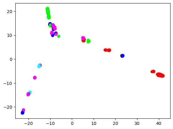
Each dot is a sample, colored by the sample’s super population. Overall, Europeans (blue), East Asians (green), and Africans (red) make three extremities, and Americans (cyan) and South Asians (purple) connect these three extremities. However, European dots are not clearly separated from other super population dots. Meanwhile, East Asian and African dots are more clearly separated. This is understandable, because the European super population in the 1000 Genomes Project includes British, Spanish, Finnish, Italian, and people of Northern and Western European ancestry, so it is already quite diverse. We will see if trained classifiers will reflect this aspect.
Training and testing classifiers
The first kind of classifiers we will test is K-nearest neighbor (k-NN) classifier.
from sklearn.neighbors import KNeighborsClassifier
from sklearn.model_selection import train_test_split

clf = KNeighborsClassifier()
y = superpopulations
X_train, X_test, y_train, y_test = train_test_split(X, y)
y_pred = clf.fit(X_train, y_train).predict(X_test)
This classifier’s precision, accuracy, and F1 score are:
     Precision  F1 score
AFR  0.924      0.912
AMR  0.548      0.430
EAS  0.962      0.971
EUR  0.532      0.596
SAS  0.838      0.844

Accuracy: 0.773
Good performance with Africans and East Asians and lower performance with Europeans agree with what we saw in the PCA plot in the previous section.
The next is Random Forest classifier.
from sklearn.ensemble import RandomForestClassifier
from sklearn.model_selection import train_test_split

clf = RandomForestClassifier(n_estimators=10)
y = superpopulations
X_train, X_test, y_train, y_test = train_test_split(X, y)
y_pred = clf.fit(X_train, y_train).predict(X_test)
This classifier’s precision, accuracy, and F1 score are:
     Precision  F1 score
AFR  0.944      0.944
AMR  0.478      0.543
EAS  0.981      0.981
EUR  0.642      0.602
SAS  0.924      0.897

Accuracy: 0.825
This one performs slightly better than the k-NN one, but it has the same characteristic that it performs better with Africans and East Asians than with Europeans.
Epilog
get_sample_uid_variant_arrays can be used to selectively retrieve samples and variants.
samples, uids, variants = get_sample_uid_variant_arrays(
    "ALL.chrY.phase3_integrated_v2b.20130502.genotypes.vcf.sqlite",
    variant_criteria="gnomad3__af > 0.01"
)
will return variants the gnomAD allele frequency of which is greater than 1%, if the input file was annotated with gnomad3 OakVar module as in
ov run ALL.chrY.phase3_integrated_v2b.20130502.genotypes.vcf.sqlite -a gnomad3
samples and uids will be adjusted accordingly as well. Any OakVar module can be used for such filtration.
This was a quick demonstration of OakVar’s ability to interface genomic data and scikit-learn, a machine learning framework. Please stay tuned for future publications for more examples.